

Introducing the basic concepts of statistical analysis,cornerstone of data science. Available both in PDF(more graphs and tables) and web form.
Statistical analysis allows a better understanding of the basic structure of the data and carry out a number of procedures to identify possible correlations between variables, recognize trends and, as an integral part of a data mining tool enable predictions. Below we present two main features of a statistical analysis
• Crosstabulation.
• Descriptive Statistics.
1 ) Types of Variables
The variables typically used in statistical analysis fall into one of the following three basic categories.
1.1 Arithmetic (or Quantitative or Scale) Variables
These variables take values in an interval of the real line and include the height, weight or income of an individual, the distance traveled by some automobile, the life-span of a machine, etc.
1.2 Categorical (or Qualitative or Nominal) Variables
These variables record qualitative attributes of the objects under consideration. Usually the possible categories are called the levels of the nominal variable. Examples of categorical variables include the political preference (Right, Center, Left), the preferred kind of music (Rock, Jazz, Classical, Country, Folk, etc.), the grade of a student in some exam (A, B, C, D, F), etc.
1.3 Ordinal Variables
These are nominal variables whose levels can be ordered in some logical sense, however the distances between the various levels are not exactly known. Examples of ordinal variables include the age group of an individual (teenager, middle aged, old), the opinion on some matter (absolutely disagree, disagree, rather disagree, rather agree, agree, absolutely agree), the grade of a student in some exam (A, B, C, D, F), etc.
2) Frequency Tables
A frequency table is a table that lists items and uses tally marks to record and show the number of times they occur. Each entry of such a table contains the frequency or count of the occurrences of values within a particular group or interval, and in this way, the table summarizes the distribution of values in the sample. Frequency tables can be used for any dependent (e.g. answer to a poll question) or independent (e.g. age, gender, etc.) variable. It is often useful that percentages are included, taking into account the missing values
3) Crosstabs or Contingency Tables
Cross-tabulation is the process of creating a table from the multivariate frequency distribution of two statistical variables, tabulating the results of one variable against the other. Such tables are called contingency tables and give a basic picture of the interrelation of the two variables. In contingency tables, independent variables (e.g. the gender) are usually displayed as rows and dependent variables (e.g. an answer to a poll question) as columns. It is often useful that percentages by row, by column, or total percentages are included . Contingency tables can analogously be defined for three or more variables, however for more than three variables they are hard to use and are usually avoided.
4) Pearson chi-square (χ2) test
This test is used for contingency tables and tests whether two categorical variables are dependent or not. For example, one can check whether the answer to the question ”Do you agree with Newsweek’s cover suggesting that Obama must go?” depends on the gender or age of the person responding. This test makes use of a test Statistic proposed by Carl Pearson in 1900, which is a function of the squares of the deviations of the observed counts from their expected values, weighted by the reciprocals of their expected values.
5) Descriptives
Descriptive measures make sense for statistical analysis of quantitative data and include the following:
5.1 The Central Tendency
The central tendency includes Statistics which describe the location of the distribution of a quantitative variable. It includes the mean, the median, and the sum.
• The Mean is the arithmetic average i.e. the sum of values of the quantitative variable divided by the number of cases.
• The Median is the value above and below which half of the cases fall. It is also called the 50th percentile. If there is an even number of cases, the median equals the average of the two middle cases when they are sorted in ascending or descending order, while in an odd number of cases it equals the middle case, when the cases are sorted as above. The median is a measure of central tendency not
sensitive to outlying values (unlike the mean, which can be affected by a few extremely high or low values).
• The Sum equals the sum of the values across all cases with non-missing values.
5.2 The Dispersion
The dispersion includes Statistics which measure the amount of variation or spread in the data. They include the standard deviation, the variance, the range, the minimum, the maximum, and the standard error of the mean.
- The Standard deviation is a measure of dispersion around the mean. In any distribution, 93.75% of the cases fall within four standard deviation of the mean (Chebyshev’s inequality). In a normal distribution, 68% of cases fall within one standard deviation of the mean and 95% of cases fall within two standard deviations. For example, if the mean age is 45 years with a standard deviation of 10 years, in a normal distribution, 95% of the cases will have to be between 25 and 65 years of age.
- The Variance measures the amount of variation around the mean and is equal to the sum of squared deviations from the mean divided by one less than the number of cases. The variance is measured in units that are the square of those of the variable itself.
- The Range equals the difference between the largest and smallest values of a quantitative variable.
- The Minimum is the smallest value of a quantitative variable.
- The Maximum is the largest value of a quantitative variable.
- The Standard Error of the Mean measures how much the value of the mean may vary from sample to sample taken from the same distribution and can be used to roughly compare the observed mean to a hypothesized value.
5.3 The Distribution
The distribution includes the skewness and kurtosis which are Statistics describing the shape and symmetry of the distribution. These statistics are displayed with their standard errors.
- The Skewness is a measure of the asymmetry of a distribution. The normal distribution is symmetric and has zero skewness. Distributions with a significant positive skewness have a long right tail while distributions with a significant negative skewness have a long left tail. As a guideline, a skewness value more than twice its standard error is taken to indicate departure from symmetry
- The Kurtosis is a measure of the extent to which observations cluster around a central point. Positive kurtosis indicates that, relative to a normal distribution of the same mean and variance, the obser- vations are more clustered about the center of the distribution and have thinner tails towards the extreme values of the distribution. At these points, the tails of leptokurtic distributions are thicker relative to a normal distribution. Negative kurtosis indicates that, relative to a normal distribution of the same mean and variance, the observations cluster less and have thicker tails towards the extreme values of the distribution. At these point, the tails of platykurtic distributions are thinner relative to a normal distribution
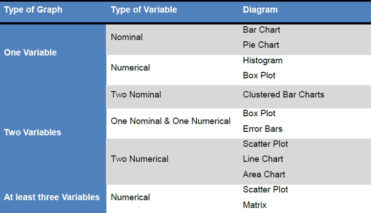
5.5 Graphs
Graphs enable us to understand the relationship between variables, and interpret the behavior of objects under consideration in a simple, pictorial way, easily understood by almost everyone.
In the following table we present a list of graphs suitable for the study of variables or combinations of variables of specific type.
AI ANALYTICS DATA DATA ANALYTICS DATA SCIENCE GRAPHS MACHINE LEARNING VISUALIZATIONS
